Shapley computes feature contributions for single predictions with the
Shapley value, an approach from cooperative game theory. The features values
of an instance cooperate to achieve the prediction. The Shapley value fairly
distributes the difference of the instance's prediction and the datasets
average prediction among the features.
Details
For more details on the algorithm see https://christophm.github.io/interpretable-ml-book/shapley.html
References
Strumbelj, E., Kononenko, I. (2014). Explaining prediction models and individual predictions with feature contributions. Knowledge and Information Systems, 41(3), 647-665. https://doi.org/10.1007/s10115-013-0679-x
See also
Shapley
A different way to explain predictions: LocalModel
Super class
iml::InterpretationMethod -> Shapley
Public fields
x.interestdata.frame
Single row with the instance to be explained.y.hat.interestnumeric
Predicted value for instance of interest.y.hat.averagenumeric(1)
Average predicted value for dataX.sample.sizenumeric(1)
The number of times coalitions/marginals are sampled from data X. The higher the more accurate the explanations become.
Methods
Inherited methods
Method new()
Create a Shapley object
Usage
Shapley$new(predictor, x.interest = NULL, sample.size = 100)Arguments
predictorPredictor
The object (created withPredictor$new()) holding the machine learning model and the data.x.interestdata.frame
Single row with the instance to be explained.sample.sizenumeric(1)
The number of Monte Carlo samples for estimating the Shapley value.
Returns
data.frame
data.frame with the Shapley values (phi) per feature.
Method explain()
Set a new data point which to explain.
Arguments
x.interestdata.frame
Single row with the instance to be explained.
Examples
library("rpart")
# First we fit a machine learning model on the Boston housing data
data("Boston", package = "MASS")
rf <- rpart(medv ~ ., data = Boston)
X <- Boston[-which(names(Boston) == "medv")]
mod <- Predictor$new(rf, data = X)

# Then we explain the first instance of the dataset with the Shapley method:
x.interest <- X[1, ]
shapley <- Shapley$new(mod, x.interest = x.interest)
shapley
#> Interpretation method:  Shapley
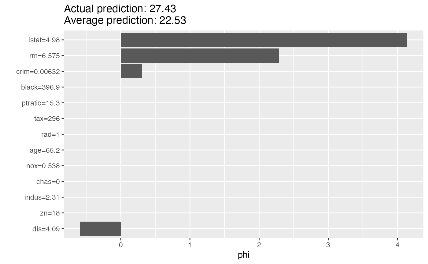
#> Predicted value: 27.427273, Average prediction: 22.532806 (diff = 4.894466)
#>
#> Analysed predictor:
#> Prediction task: unknown
#>
#>
#> Analysed data:
#> Sampling from data.frame with 506 rows and 13 columns.
#>
#>
#> Head of results:
#>   feature       phi   phi.var feature.value
#> 1    crim 0.3095547  1.516409  crim=0.00632
#> 2      zn 0.0000000  0.000000         zn=18
#> 3   indus 0.0000000  0.000000    indus=2.31
#> 4    chas 0.0000000  0.000000        chas=0
#> 5     nox 0.0000000  0.000000     nox=0.538
#> 6      rm 2.2868013 23.014323      rm=6.575

# Look at the results in a table
shapley$results
#>    feature        phi   phi.var feature.value
#> 1     crim  0.3095547  1.516409  crim=0.00632
#> 2       zn  0.0000000  0.000000         zn=18
#> 3    indus  0.0000000  0.000000    indus=2.31
#> 4     chas  0.0000000  0.000000        chas=0
#> 5      nox  0.0000000  0.000000     nox=0.538
#> 6       rm  2.2868013 23.014323      rm=6.575
#> 7      age  0.0000000  0.000000      age=65.2
#> 8      dis -0.5863443  6.867283      dis=4.09
#> 9      rad  0.0000000  0.000000         rad=1
#> 10     tax  0.0000000  0.000000       tax=296
#> 11 ptratio  0.0000000  0.000000  ptratio=15.3
#> 12   black  0.0000000  0.000000   black=396.9
#> 13   lstat  4.1406006 38.654545    lstat=4.98
# Or as a plot
plot(shapley)


# Explain another instance
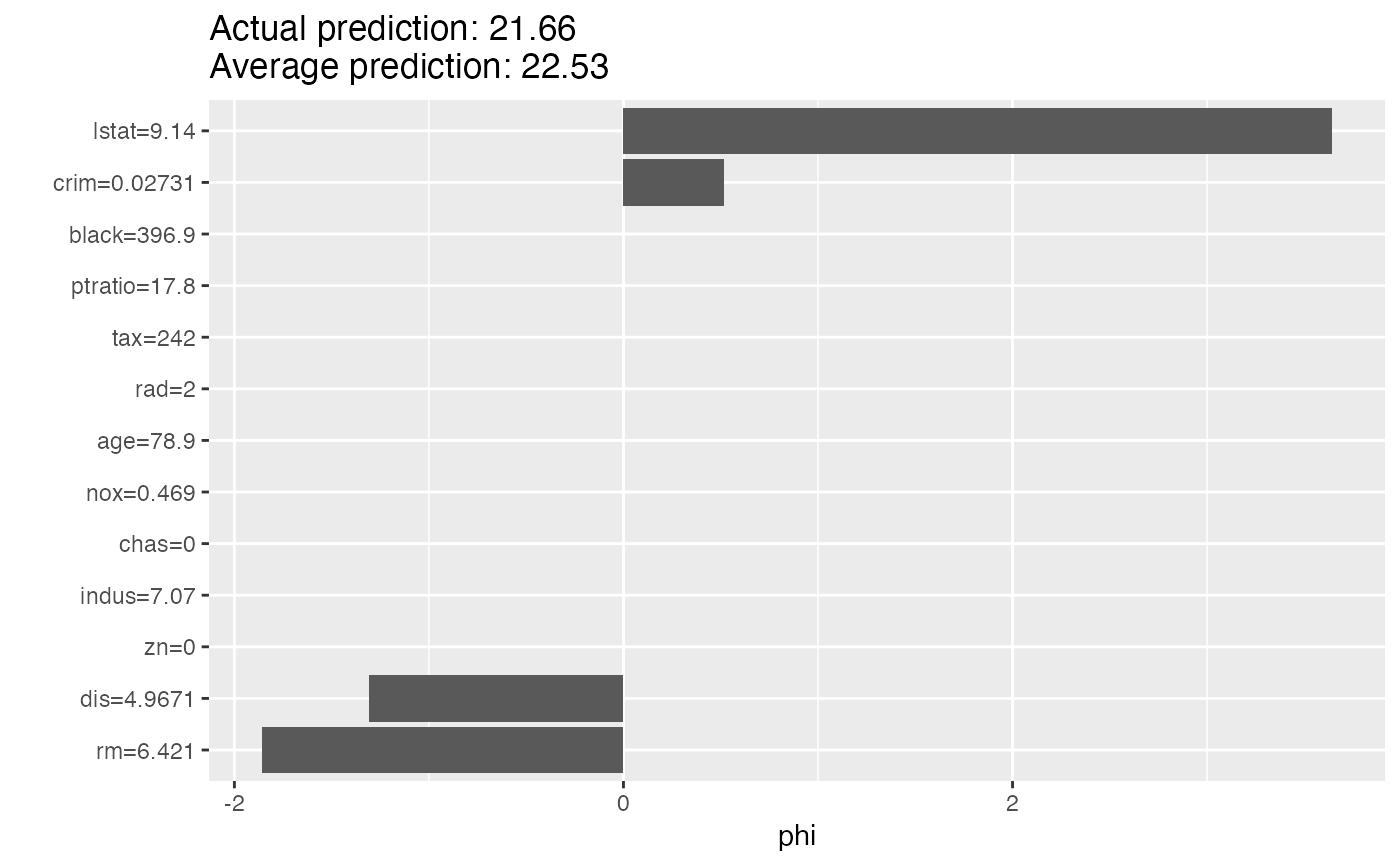
shapley$explain(X[2, ])
plot(shapley)

if (FALSE) { # \dontrun{
# Shapley() also works with multiclass classification
rf <- rpart(Species ~ ., data = iris)
X <- iris[-which(names(iris) == "Species")]
mod <- Predictor$new(rf, data = X, type = "prob")

# Then we explain the first instance of the dataset with the Shapley() method:
shapley <- Shapley$new(mod, x.interest = X[1, ])
shapley$results
plot(shapley)

# You can also focus on one class
mod <- Predictor$new(rf, data = X, type = "prob", class = "setosa")
shapley <- Shapley$new(mod, x.interest = X[1, ])
shapley$results
plot(shapley)
} # }