Effect of a feature on predictions

FeatureEffect computes and plots (individual) feature effects of prediction models.

Details

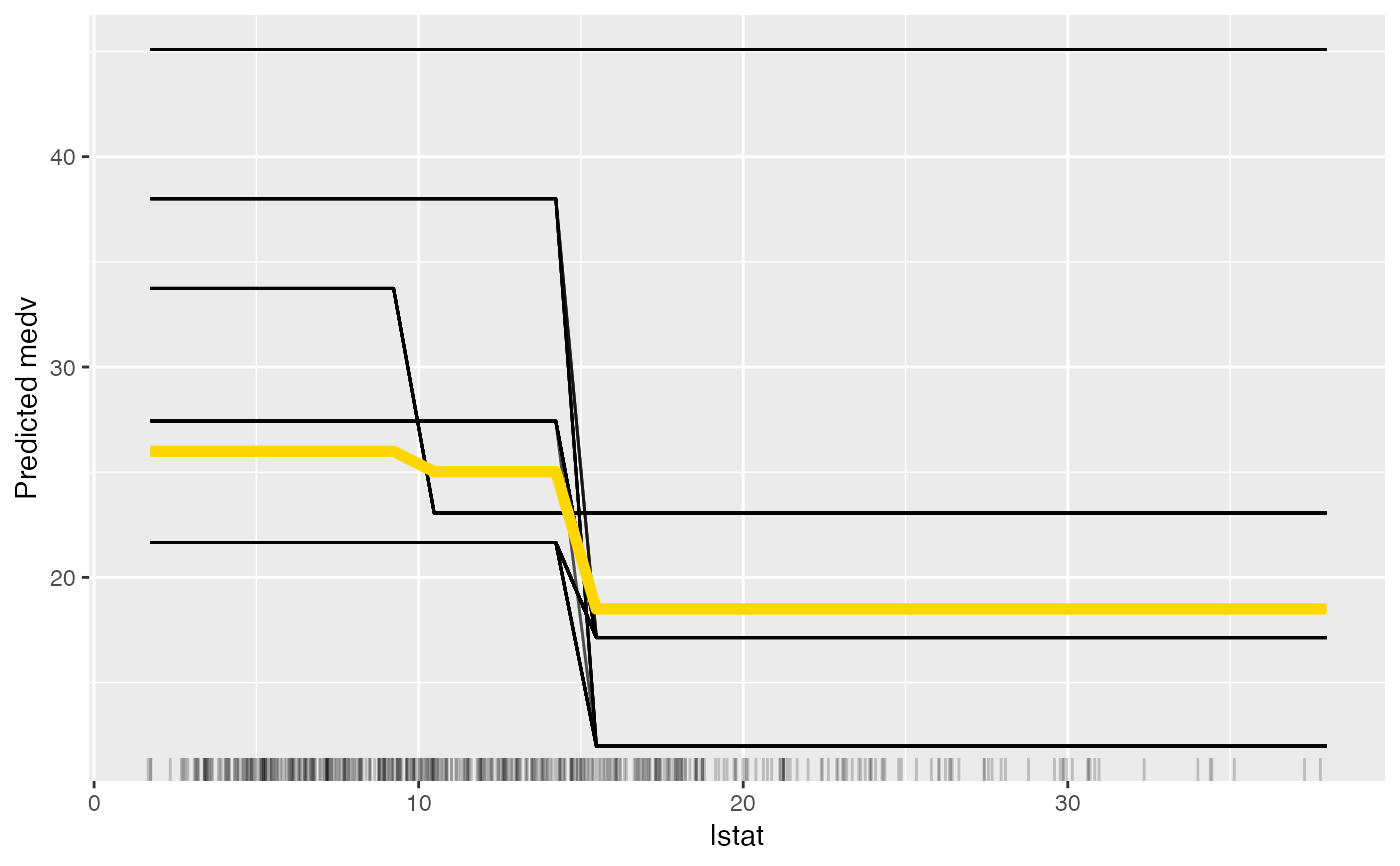
The FeatureEffect class compute the effect a feature has on the prediction. Different methods are implemented:

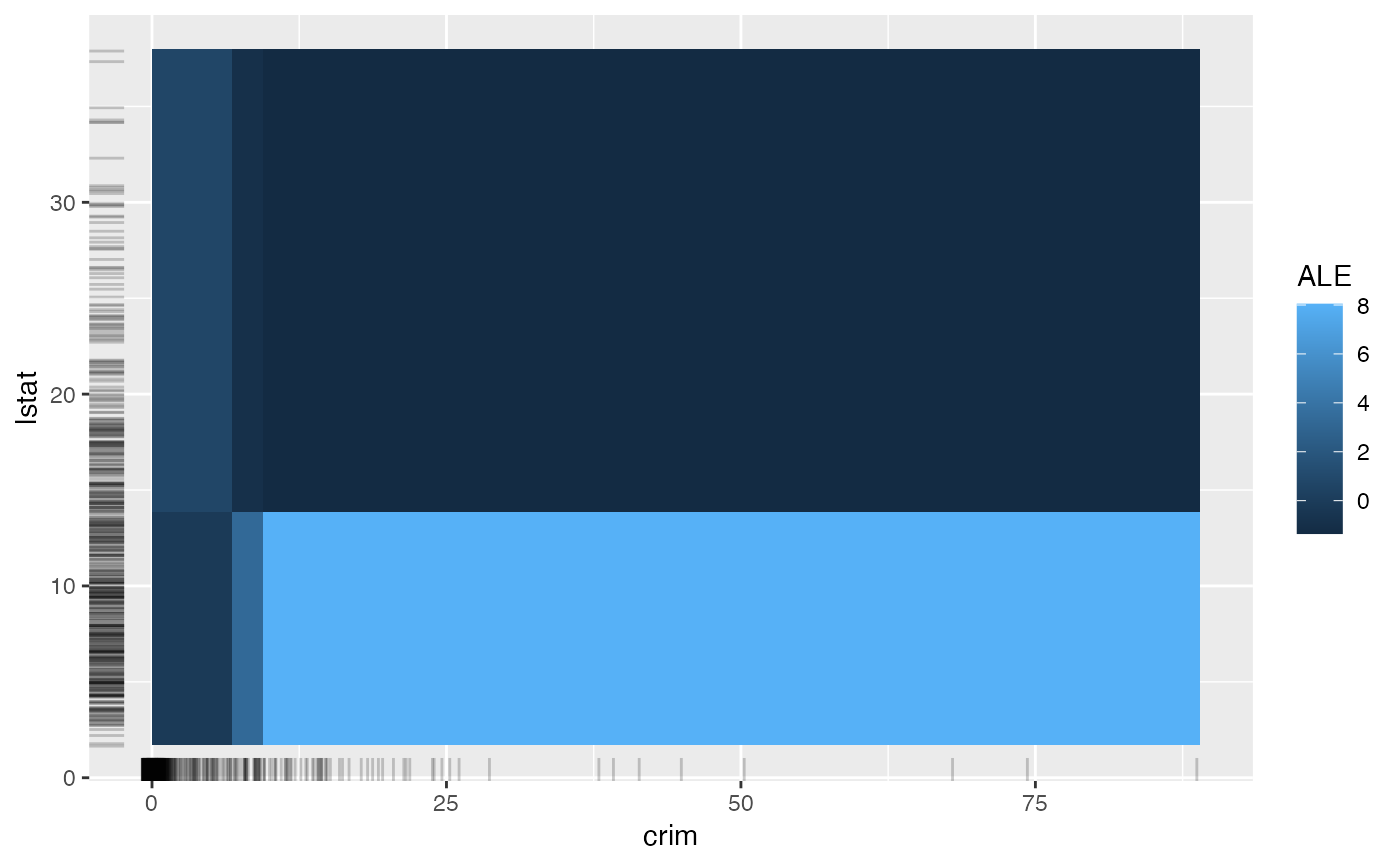
Accumulated Local Effect (ALE) plots
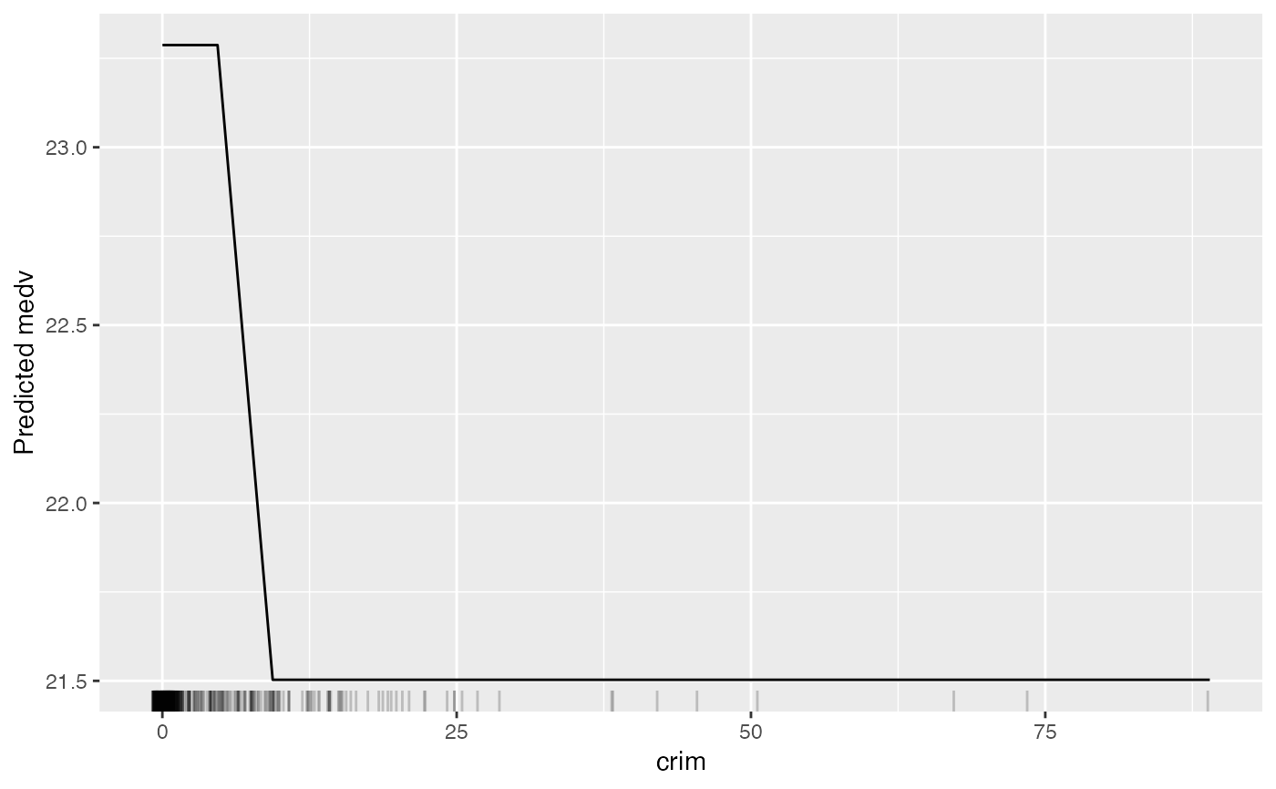
Partial Dependence Plots (PDPs)
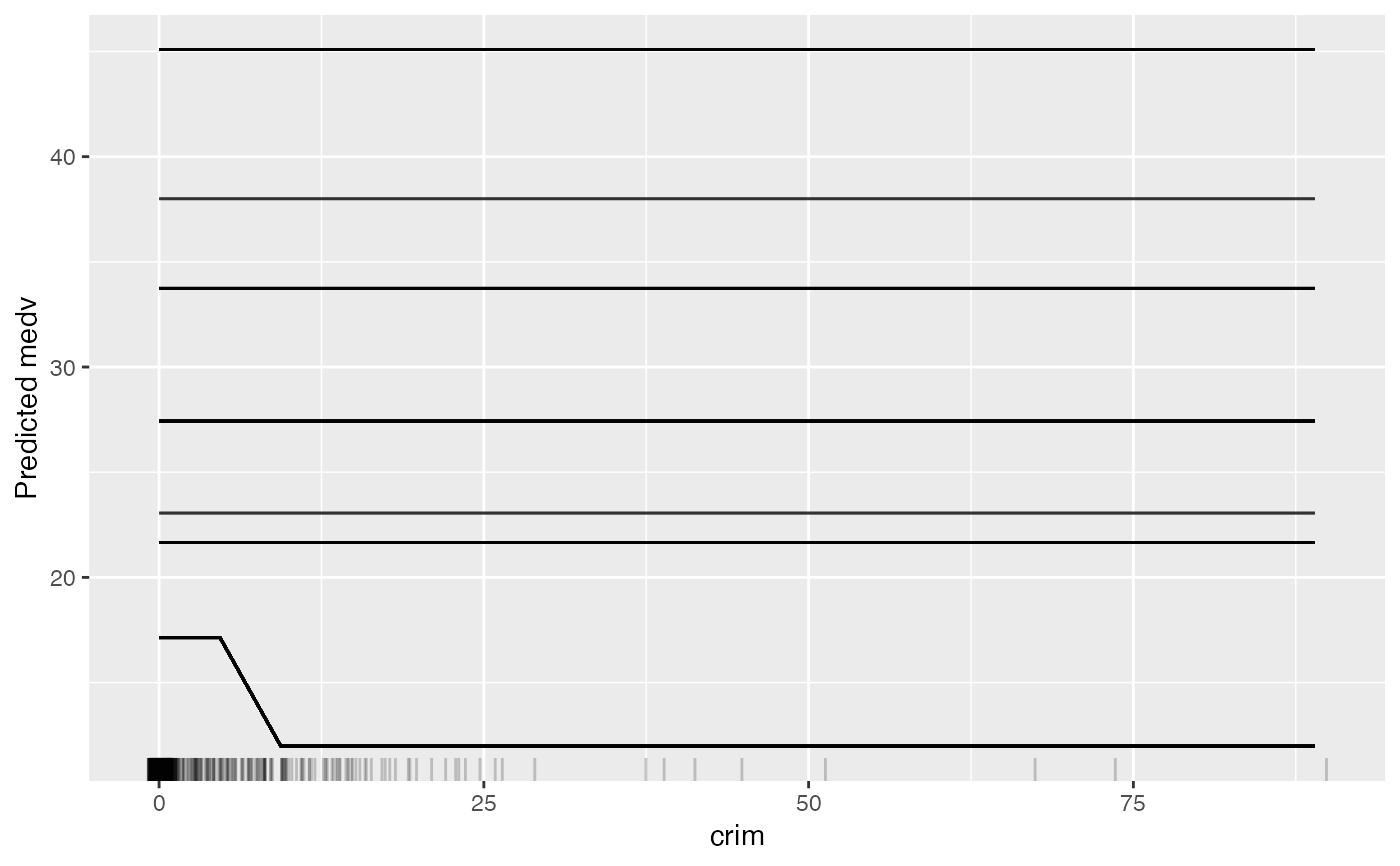
Individual Conditional Expectation (ICE) curves

Accumulated local effects and partial dependence plots both show the average model prediction over the feature. The difference is that ALE are computed as accumulated differences over the conditional distribution and partial dependence plots over the marginal distribution. ALE plots preferable to PDPs, because they are faster and unbiased when features are correlated.

ALE plots for categorical features are automatically ordered by the similarity of the categories based on the distribution of the other features for instances in a category. When the feature is an ordered factor, the ALE plot leaves the order as is.

Individual conditional expectation curves describe how, for a single observation, the prediction changes when the feature changes and can be combined with partial dependence plots.

To learn more about accumulated local effects, read the Interpretable Machine Learning book.

For the partial dependence plots: https://christophm.github.io/interpretable-ml-book/pdp.html

For individual conditional expectation: https://christophm.github.io/interpretable-ml-book/ice.html

References

Apley, D. W. 2016. "Visualizing the Effects of Predictor Variables in Black Box Supervised Learning Models." ArXiv Preprint.

Friedman, J.H. 2001. "Greedy Function Approximation: A Gradient Boosting Machine." Annals of Statistics 29: 1189-1232.

Goldstein, A., Kapelner, A., Bleich, J., and Pitkin, E. (2013). Peeking Inside the Black Box: Visualizing Statistical Learning with Plots of Individual Conditional Expectation, 1-22. https://doi.org/10.1080/10618600.2014.907095

Super class

iml::InterpretationMethod -> FeatureEffect

Public fields

grid.size: (numeric(1) | numeric(2))
The size of the grid.
feature.name: (character(1) | character(2))
The names of the features for which the partial dependence was computed.
n.features: (numeric(1))
The number of features (either 1 or 2).
feature.type: (character(1) | character(2))
The detected types of the features, either "categorical" or "numerical".
method: (character(1))

Active bindings

center.at: numeric
Value at which the plot was centered. Ignored in the case of two features.

Methods

Inherited methods

Method `new()`

Create a FeatureEffect object

Usage

FeatureEffect$new(
  predictor,
  feature,
  method = "ale",
  center.at = NULL,
  grid.size = 20,
  grid.points = NULL
)

Arguments

predictor

Predictor
The object (created with Predictor$new()) holding the machine learning model and the data.

feature

(character(1) | character(2) | numeric(1) | numeric(2))
The feature name or index for which to compute the effects.

method

(character(1))

'ale' for accumulated local effects,
'pdp' for partial dependence plot,
'ice' for individual conditional expectation curves,
'pdp + ice' for partial dependence plot and ice curves within the same plot.

center.at

(numeric(1))
Value at which the plot should be centered. Ignored in the case of two features.

grid.size

(numeric(1) | numeric(2))
The size of the grid for evaluating the predictions.

grid.points

(numeric() | list(numeric(), numeric())
An optional grid along the feature. If grid.points are set, the grid.size argument is ignored. Provide a list of two vectors with the same order as in the 'feature' argument, if PDP/ALE for two features is to be computed with a user-defined grid.

Method `set.feature()`

Get/set feature(s) (by index) for which to compute PDP.

Usage

FeatureEffect$set.feature(feature)

Arguments

feature: (character(1))
Feature name.

Method `center()`

Set the value at which the ice computations are centered.

Usage

FeatureEffect$center(center.at)

Arguments

center.at: (numeric(1))
Value at which the plot should be centered. Ignored in the case of two features.

Method `predict()`

Predict the marginal outcome given a feature.

Usage

FeatureEffect$predict(data, extrapolate = FALSE)

Arguments

data: data.frame
Data.frame with the feature or a vector.
extrapolate: (character(1))
If TRUE, predict returns NA for x values outside of observed range. If FALSE, predcit returns the closest PDP value for x values outside the range. Ignored for categorical features

Returns

Values of the effect curves at the given values.

Method `clone()`

The objects of this class are cloneable with this method.

Usage

FeatureEffect$clone(deep = FALSE)

Arguments

deep: Whether to make a deep clone.

Examples

# We train a random forest on the Boston dataset:
data("Boston", package = "MASS")
library("rpart")
rf <- rpart(medv ~ ., data = Boston)
mod <- Predictor$new(rf, data = Boston)

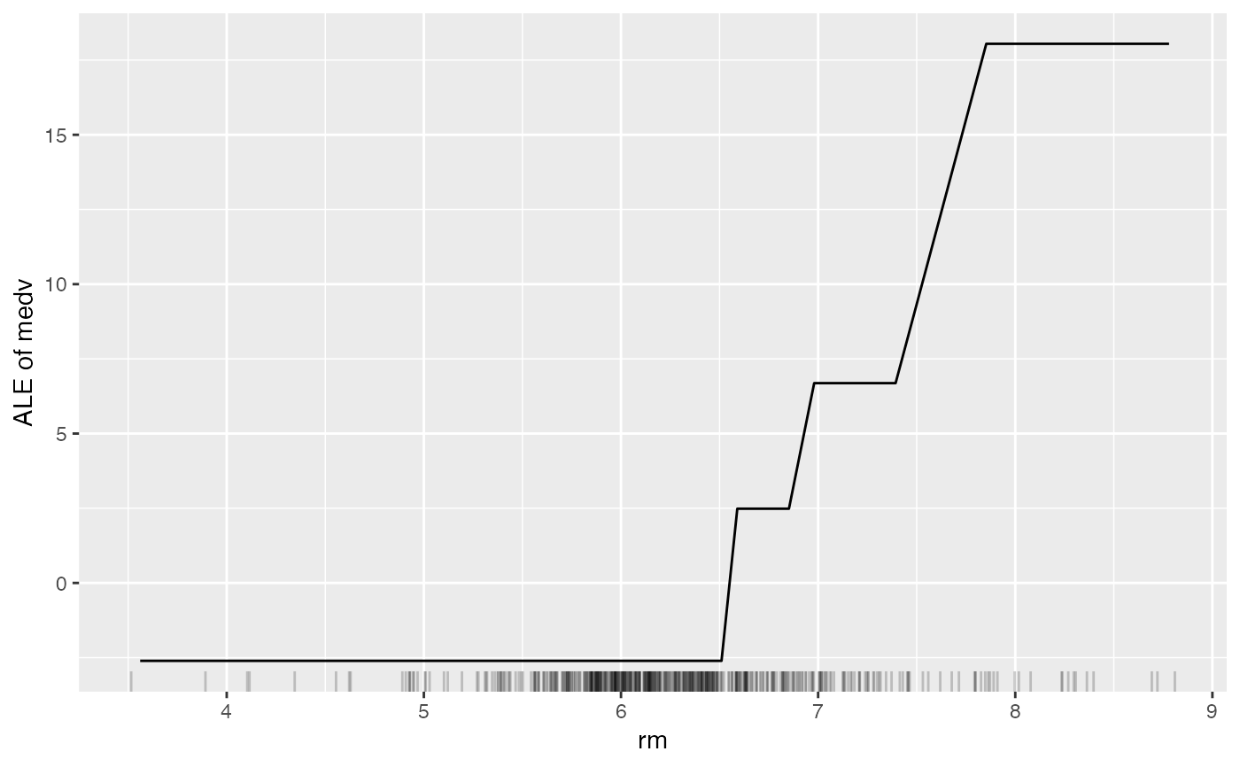
# Compute the accumulated local effects for the first feature
eff <- FeatureEffect$new(mod, feature = "rm", grid.size = 30)
eff$plot()


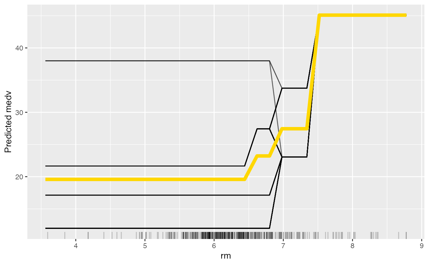
# Again, but this time with a partial dependence plot and ice curves
eff <- FeatureEffect$new(mod,
  feature = "rm", method = "pdp+ice",
  grid.size = 30
)
plot(eff)


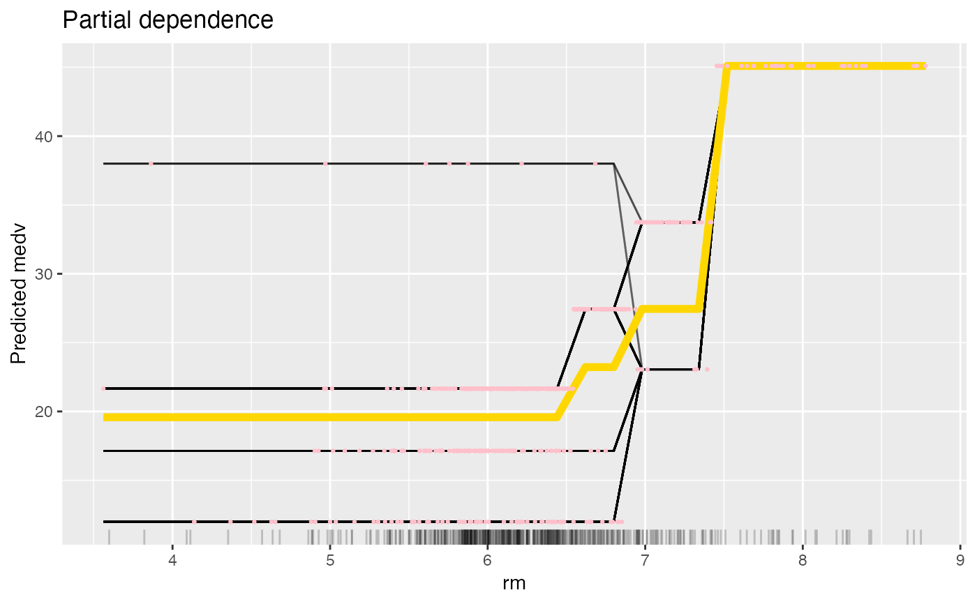
# Since the result is a ggplot object, you can extend it:
library("ggplot2")
plot(eff) +
  # Adds a title
  ggtitle("Partial dependence") +
  # Adds original predictions
  geom_point(
    data = Boston, aes(y = mod$predict(Boston)[[1]], x = rm),
    color = "pink", size = 0.5
  )


# If you want to do your own thing, just extract the data:
eff.dat <- eff$results
head(eff.dat)
#>         rm   .value .type .id
#> 1 3.561000 19.58263   pdp  NA
#> 2 3.740966 19.58263   pdp  NA
#> 3 3.920931 19.58263   pdp  NA
#> 4 4.100897 19.58263   pdp  NA
#> 5 4.280862 19.58263   pdp  NA
#> 6 4.460828 19.58263   pdp  NA

# You can also use the object to "predict" the marginal values.
eff$predict(Boston[1:3, ])
#> [1] 22.30267 19.58263 27.44788
# Instead of the entire data.frame, you can also use feature values:
eff$predict(c(5, 6, 7))
#> [1] 19.58263 19.58263 27.44788

# You can reuse the pdp object for other features:
eff$set.feature("lstat")
plot(eff)


# Only plotting the aggregated partial dependence:
eff <- FeatureEffect$new(mod, feature = "crim", method = "pdp")
eff$plot()


# Only plotting the individual conditional expectation:
eff <- FeatureEffect$new(mod, feature = "crim", method = "ice")
eff$plot()


# Accumulated local effects and partial dependence plots support up to two
# features:
eff <- FeatureEffect$new(mod, feature = c("crim", "lstat"))
#> Warning: Unknown argument 'on' has been passed.
#> Loading required namespace: yaImpute
#> Warning: Unknown argument 'on' has been passed.
plot(eff)


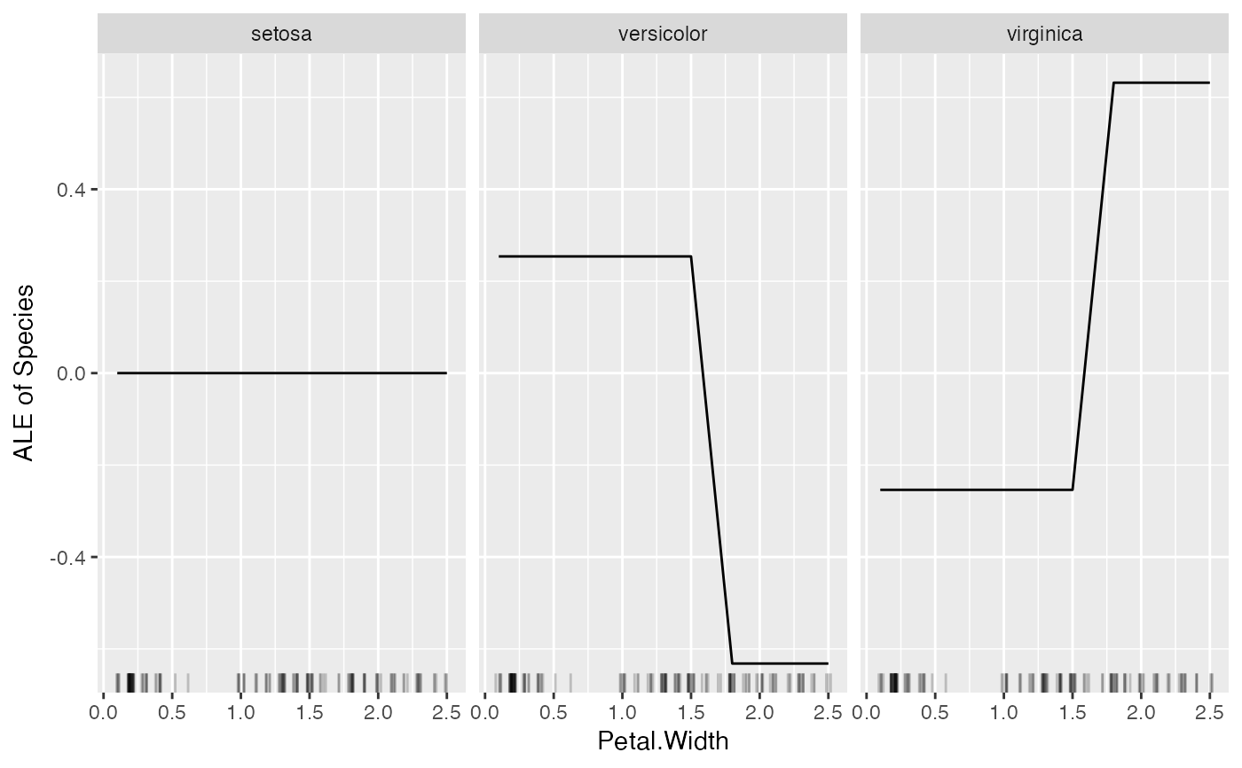
# FeatureEffect plots also works with multiclass classification
rf <- rpart(Species ~ ., data = iris)
mod <- Predictor$new(rf, data = iris, type = "prob")

# For some models we have to specify additional arguments for the predict
# function
plot(FeatureEffect$new(mod, feature = "Petal.Width"))


# FeatureEffect plots support up to two features:
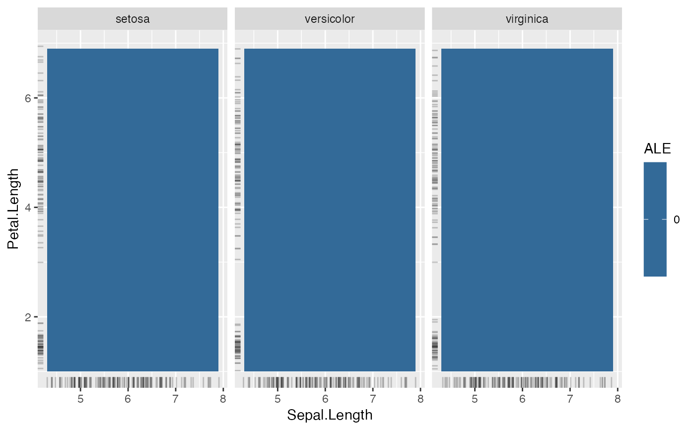
eff <- FeatureEffect$new(mod, feature = c("Sepal.Length", "Petal.Length"))
#> Warning: Unknown argument 'on' has been passed.
#> Warning: Unknown argument 'on' has been passed.
eff$plot()


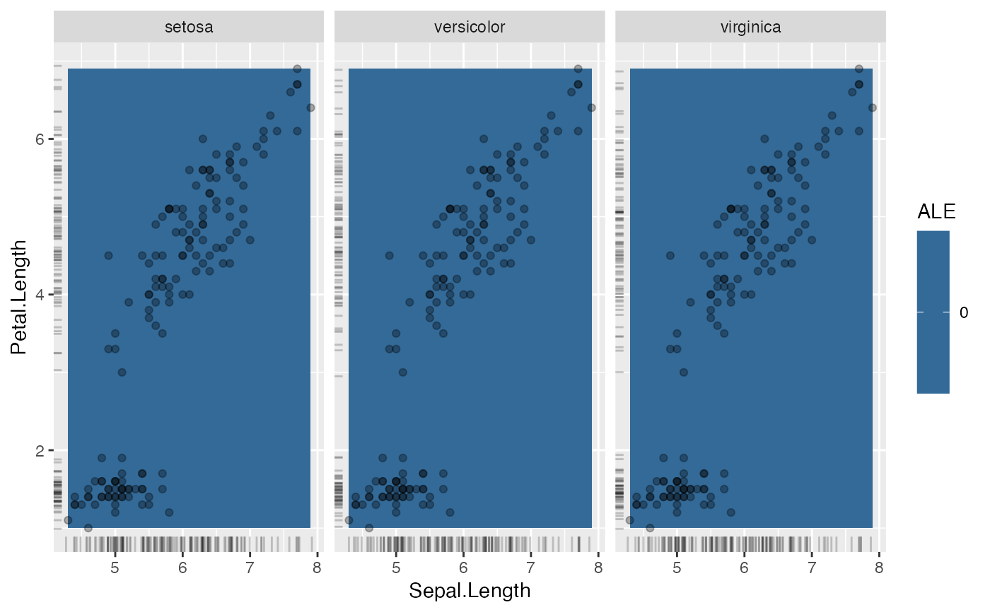
# show where the actual data lies
eff$plot(show.data = TRUE)


# For multiclass classification models, you can choose to only show one class:
mod <- Predictor$new(rf, data = iris, type = "prob", class = "setosa")
plot(FeatureEffect$new(mod, feature = "Sepal.Length"))